Profiling¶

It is virtually impossible to optimize any system without measuring its performance and identifying the bottlenecks. This guide will show you how to profile your RL workload in different regimes.

Profiling with the built-in "Timing" tool¶

Sample Factory provides a simple class called Timing (see sample_factory/utils/timing.py) that can be used for high-level profiling to get a rough idea of where the compute cycles are spent.

Core hotspots are already instrumented, but if you'd like to see a more elaborate picture, you can use the Timing class in your own code like this:

import time

timing = Timing(name="MyProfile")

# add_time() will accumulate time spent in the block
# this is the most commonly used method
with timing.add_time("hotspot"):
    # do something
    ...

    # measure time spent in a subsection of code
    # when we build the timing report, we'll generate a tree corresponding to the nesting
    with timing.add_time("subsection1"):
        # do something
        ...

    with timing.add_time("subsection2"):
        # do something
        ...

# instead of accumulating time, this will measure the last time the block was executed
with timing.timeit("hotspot2"):
    # do something
    ...

# this will measure the average time spent in the block
with timing.time_avg("hotspot3"):
    # do something
    ...

# this will print the timing report
print(timing)

Example: profiling an asynchronous workload¶

Let's take a look at a typical RL workload: training an agent in a VizDoom pixel-based environment. We use the following command line and run it on a 6-core laptop with hyperthreading:

python -m sf_examples.vizdoom.train_vizdoom --env=doom_benchmark --env_frameskip=4 --train_for_env_steps=4000000 \\
--use_rnn=True --num_workers=12 --num_envs_per_worker=16 --num_policies=1 --num_epochs=1 --rollout=32 --recurrence=32 \\
--batch_size=2048 --experiment=profiling --benchmark=True --decorrelate_envs_on_one_worker=False --res_w=128 --res_h=72 \\
--wide_aspect_ratio=True --policy_workers_per_policy=1 --worker_num_splits=2 --batched_sampling=False \\
--serial_mode=False --async_rl=True --policy_workers_per_policy=1

If we wait for this experiment to finish (in this case, after training for 4M env steps), we'll get the following timing report:

[2022-11-25 01:36:52,563][15762] Batcher 0 profile tree view:
batching: 10.1365, releasing_batches: 0.0136
[2022-11-25 01:36:52,564][15762] InferenceWorker_p0-w0 profile tree view:
wait_policy: 0.0022
  wait_policy_total: 93.7697
update_model: 2.3025
  weight_update: 0.0015
one_step: 0.0034
  handle_policy_step: 105.2299
    deserialize: 7.4926, stack: 0.6621, obs_to_device_normalize: 29.3540, forward: 38.4143, send_messages: 5.9522
    prepare_outputs: 18.2651
      to_cpu: 11.2702
[2022-11-25 01:36:52,564][15762] Learner 0 profile tree view:
misc: 0.0024, prepare_batch: 8.0517
train: 28.5942
  epoch_init: 0.0037, minibatch_init: 0.0038, losses_postprocess: 0.1654, kl_divergence: 0.2093, after_optimizer: 12.5617
  calculate_losses: 10.2242
    losses_init: 0.0021, forward_head: 0.4746, bptt_initial: 7.5225, tail: 0.3432, advantages_returns: 0.0976, losses: 0.7113
    bptt: 0.9616
      bptt_forward_core: 0.9263
  update: 5.0903
    clip: 0.8172
[2022-11-25 01:36:52,564][15762] RolloutWorker_w0 profile tree view:
wait_for_trajectories: 0.0767, enqueue_policy_requests: 5.3569, env_step: 170.3642, overhead: 10.1567, complete_rollouts: 0.3764
save_policy_outputs: 6.6260
  split_output_tensors: 3.0167
[2022-11-25 01:36:52,564][15762] RolloutWorker_w11 profile tree view:
wait_for_trajectories: 0.0816, enqueue_policy_requests: 5.5298, env_step: 169.3195, overhead: 10.2944, complete_rollouts: 0.3914
save_policy_outputs: 6.7380
  split_output_tensors: 3.1037
[2022-11-25 01:36:52,564][15762] Loop Runner_EvtLoop terminating...
[2022-11-25 01:36:52,565][15762] Runner profile tree view:
main_loop: 217.4041
[2022-11-25 01:36:52,565][15762] Collected {0: 4014080}, FPS: 18463.7

First thing to notice here: instead of a single report we have reports from all different types of components of our system: Batcher, InferenceWorker, Learner, RolloutWorker, Runner (main loop). There are 12 rollout workers but we see only 0^th (first) and 11^th (last) workers in the report - that's just to save space, reports from all other workers will be very similar.

Total training time took 217 seconds at ~18400FPS (actual FPS reported during training was ~21000FPS, but this final number takes initialization time into account).

Each individual report is a tree view of the time spent in different hotspots. For example, learner profile looks like this:

train: 28.5942
  epoch_init: 0.0037, minibatch_init: 0.0038, losses_postprocess: 0.1654, kl_divergence: 0.2093, after_optimizer: 12.5617
  calculate_losses: 10.2242
    losses_init: 0.0021, forward_head: 0.4746, bptt_initial: 7.5225, tail: 0.3432, advantages_returns: 0.0976, losses: 0.7113
    bptt: 0.9616
      bptt_forward_core: 0.9263
  update: 5.0903
    clip: 0.8172

train is the highest-level profiler context. On the next line we print all sub-profiles that don't have any sub-profiles of their own. In this case, epoch_init, minibatch_init, etc. After that, one by one, we print all sub-profiles that have sub-profiles of their own.

Let's take a look at individual component reports:

Runner (main loop) does not actually do any heavy work other than reporting summaries, so we can ignore it. It is here mostly to give us the total time from experiment start to finish.
Batcher is responsible for batching trajectories from rollout workers and feeding them to the learner. In this case it only took 10 seconds and since it was done in parallel to all other work, we can ignore it for the most part, it's pretty fast.
Learner's main hotspots took only 8 and 28 seconds. Again, considering that it was done in parallel to all other work, and the time is pretty insignificant compared to the total time of 217 seconds, we can safely say that it's not the bottleneck.
InferenceWorker's overall time is 105 seconds, which is significant. We can see that the main hotspots are forward (actual forward pass) and obs_to_device_normalize (normalizing the observations and transferring them to GPU). In order to increase throughtput we might want to make our model faster (i.e. by making it smaller) or disable normalization (parameter --normalize_input=False, see config reference). Note however that both of these measures may hurt sample efficiency.
RolloutWorkers that simulate the environment are the main culprits here. The majority of time is taken by env_step (stepping through the environment), ~170 seconds. Overall, we can say that this workload is heavily dominated by CPU-based simulation. If you're in a similar situation you might want to consider instrumenting your code deeper (i.e. using Timing or other tool) to measure hotspots in your environment and attempt to optimize it.

Notes on GPU profiling¶

Profiling GPU-based workloads can be misleading because GPU kernels are asynchronous and sometimes we can see a lot of time spent in sections after the ones we expect to be the hotspots. In the example above, the learner's after_optimizer: 12.5617 is significantly longer than update: 5.0903 where the actual backward pass happens.

Thus one should not rely too heavily on timing your code for GPU profiling. Take a look at CUDA profiling, i.e. here is a Pytorch tutorial.

Also check out this tutorial for some advanced RL profiling techniques.

Profiling with standard Python profilers (cProfile or yappi)¶

In most RL workloads in Sample Factory it can be difficult to use standard profiling tools because the full application consists of many processes and threads and in the author's experience standard tools struggle to organise traces from multiple processes into a single coherent report (if the reader knows of a good tool for this, please let the author know).

However, using serial mode we can force Sample Factory to execute everything in one process! This can be very useful for finding bottlenecks in your environment implementation without the need for manual instrumentation. The following command will run the entire experiment in a single process:

python -m sf_examples.mujoco.train_mujoco --env=mujoco_ant --serial_mode=True --async_rl=False

Note that we enable synchronous RL mode as well, it's easier to debug this way and asynchronicity does not make sense when we're not using multiple processes.

Moreover for some workloads it is actually optimal to run everything in a single process! This is true for GPU-accelerated environments such as IsaacGym or Brax. When env simulation, inference, and learning are all done on one GPU it is not necessarily beneficial to run these tasks in separate processes.

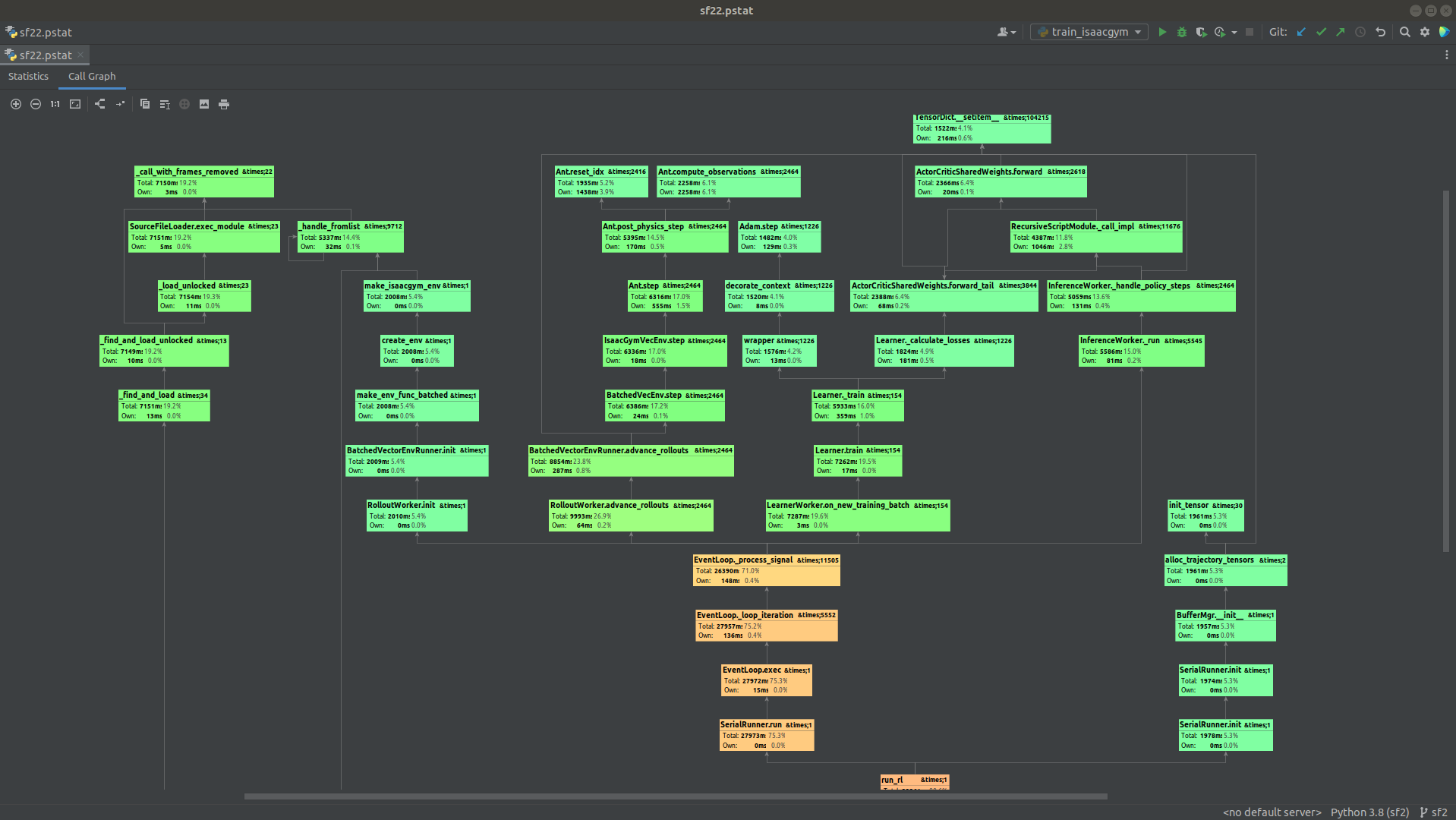
In this case we can profile Sample Factory like any other Python application. For example, PyCharm has a nice visualizer for profiling results generated by cProfile or yappi. If we run training in IsaacGym in serial mode under PyCharm's profiler:

python -m sf_examples.isaacgym_examples.train_isaacgym --env=Ant --experiment=igeAnt

we get the following report which can be explored to find hotspots in different parts of the code:

yappi profiling view